vlookup is a powerful tool that allows users to search for specific data in a large dataset. Whether you’re a business owner or simply someone who works with data, mastering the vlookup function can save you time and help you make more informed decisions.
You might be a complete beginner to vlookup. Or perhaps you’re more familiar with Excel and want to know how to execute this formula in Google Sheets.
Either way, you’ll find step-by-step instructions and useful tips below to make sure you’re using the vlookup function correctly and retrieving accurate results from your dataset.
Table of Contents
What does vlookup do in Google Sheets?
Vlookup is a function in that searches for a specific value in the leftmost column of a table or range and returns a corresponding value from a specified column within that range.
The syntax for the vlookup function is as follows:
Vlookup(search_key, range, index, [is_sorted])
- search_key is the value that you want to search for.
- range is the table or range that you want to search in.
- index is the column number (starting from 1) of the value you want to retrieve.
- is_sorted is an optional argument that indicates whether the data in the range is sorted in ascending order. If this argument is set to TRUE or omitted, the function assumes that the data is sorted and uses a faster search algorithm. If this argument is set to FALSE, the function uses a slower search algorithm that works for unsorted data.
For example, if you have a table with a list of product names in the first column and their corresponding prices in the second column, you can use the vlookup function to look up the price of a specific product based on its name.
The Benefits of Using vlookup in Google Sheets
Using vlookup can save you a lot of time when searching through large datasets. It’s a great way to quickly find the data you need without having to scroll through hundreds of rows manually.
Using vlookup in Google Sheets also:
- Saves time and effort. You can quickly retrieve information from large datasets by automating the search and retrieval process through vlookup. This can save you a lot of time and effort compared to manually searching for information in a table.
- Reduces errors. When searching for information manually, there is a risk of human error, such as mistyping or misreading information. Vlookup can help you avoid these errors by performing accurate searches based on exact matches.
- Increases accuracy. Vlookup helps ensure that you’re retrieving the correct information by allowing you to search for specific values in a table. This can help you avoid retrieving incorrect or irrelevant information.
- Improves data analysis. You can analyze data more efficiently by using vlookup to compare and retrieve data from different tables. This can help you easily identify patterns, trends, and relationships between data points.
- Provides flexibility and customization. Vlookup allows you to specify the search criteria and choose which columns to retrieve data from, making it a versatile and customizable tool that can be used for a wide range of tasks.
How to Use vlookup in Google Sheets
- Open a new or existing Google Sheet.
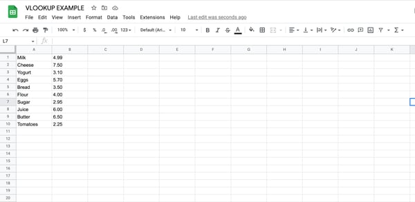
- Enter the data you want to search for in one column of the sheet. For example, you might have a list of product names in column A.
- Enter the corresponding data you want to retrieve in another column of the sheet. For example, you might have a list of prices in column B.
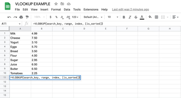
- Decide which cell you want to use to enter the vlookup formula, and click on that cell to select it.
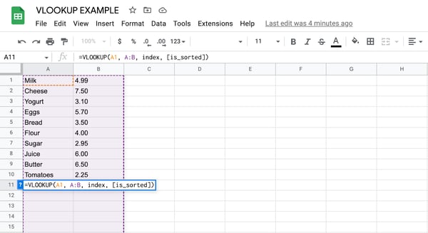
- Type the following formula into the cell:
=VLOOKUP(search_key, range, index, [is_sorted])
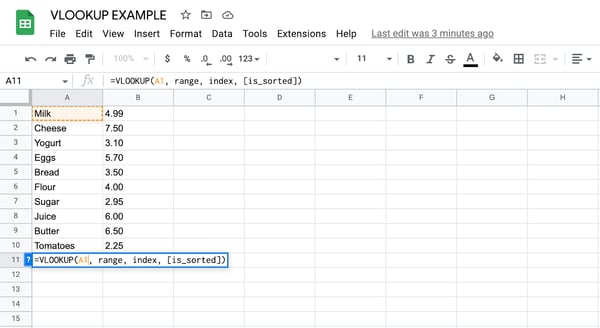
- Replace the “search_key” argument with a reference to the cell containing the value you want to search for. For example, if you want to search for the price of a product named “Milk” and “Milk” is in cell A1, you would replace “search_key” with “A1”
- Replace the “range” argument with a reference to the range of cells that contains the data you want to search in.
For example, if your product names are in column A and your prices are in column B, you would replace “range” with “A:B”.
You can also just click and drag your mouse over the range of cells the vlookup should use to retrieve the data if you’re working with a smaller dataset.
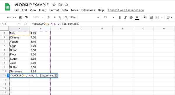
- Replace the “index” argument with the number of the column containing the data you want to retrieve. For example, if you want to retrieve prices from column B, you would replace “index” with “2”.
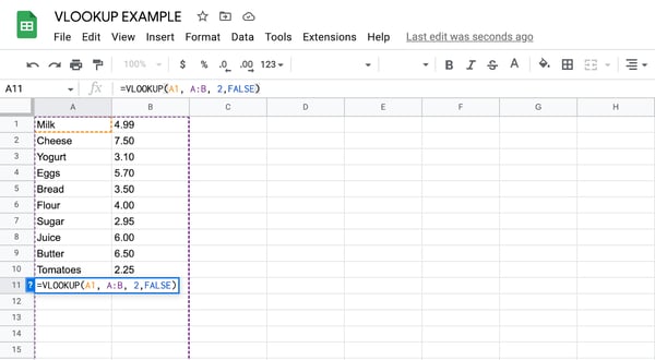
- If the data in your range is sorted in ascending order, you can omit the final “[is_sorted]” argument or set it to “TRUE”. If the data is not sorted, you should set this argument to “FALSE” to ensure accurate results.
- Press Enter to apply the formula and retrieve the desired data.
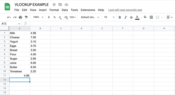
That’s it! The vlookup function should now retrieve the corresponding data based on the search key you specified. You can copy the formula to other cells in the sheet to retrieve additional data.
vlookup Example
Let’s take a look at a practical example of how to use the vlookup function in Google Sheets.
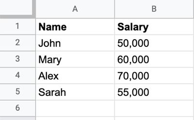
Suppose you have a table that lists the names of employees in column A and their corresponding salaries in column B. You want to look up the salary of an employee named “John” using the vlookup function.
Once the data is entered into a Google Sheet, you need to decide which cell you want to use to enter the vlookup formula, and click on that cell to select it before typing in the following formula:
=VLOOKUP(“John”, A:B, 2, FALSE)
The vlookup function should now retrieve the salary of John, which is 50,000. Here’s how the formula works:
In the first argument, “John” is the search key, which is the value you want to look up in the leftmost column of the table. In the second argument, “A:B” is the range you want to search in, which includes both columns A and B.
In the third argument, “2” is the index of the column you want to retrieve data from, which is column B (since salaries are listed in column B).
The fourth argument, “FALSE”, indicates that the data in the range is not sorted in ascending order.
So the formula searches for the name “John” in the leftmost column of the table, finds the corresponding salary in column B, and returns that value (50,000).
Best Practices for Using vlookup
There are a few key things to remember when using vlookup in Google Sheets to ensure it works properly and returns accurate data.
Make sure the data is in the same row.
First, make sure that the data you want to return is in the same row as the value you’re searching for. Otherwise, vlookup won’t be able to find it.
Sort the first column by ascending order.
Make sure that the first column of your data range is sorted in ascending order.
This will ensure that the vlookup function returns the correct results. If not, make sure you use the FALSE argument in the formula.
Include headers in the vlookup formula.
If your data range includes headers, be sure to include them in your vlookup formula so that the function knows where to find the relevant data. Otherwise, the function may not know which column to search in and could return incorrect results.
For example, if your columns have headers in Row 1 of the sheet such as “Price,” “Name,” or “Category,” make sure these cells are included in the “range” section of the formula.
Make use of the wildcard character.
The wildcard character (*) can be used in the lookup value to represent any combination of characters.
For example, suppose you have a list of product names in the first column of a data range, and you want to look up the sales for a product called “Chocolate Bar.”
However, the name of the product in the data range is listed as “Chocolate Bar – Milk Chocolate.” In this case, an exact match lookup would not find the sales for the “Chocolate Bar” product.
Here is how you would include the wildcard character in the Google Sheets vlookup formula:
=VLOOKUP(“Chocolate Bar*”, A2:B10, 2, FALSE)
It’s important to note that when using a wildcard character, vlookup will return the first match it finds in the first column of the data range that matches the lookup value.
If there are multiple matches, it will return the first one it finds. Therefore, it’s important to ensure that the lookup value is specific enough to return the desired result.
Match your formula to the case of the data you’re seeking.
Remember that vlookup is case-sensitive, so the value you enter into the formula must match the case of the value in the cells.
For example, let’s say you have a data range that includes a column of product names, and the product names are listed in different cases in different cells, such as “apple,” “Apple,” and “APPLE.”
If you’re using VLOOKUP to search for the sales of a particular product, you need to make sure that the lookup value in your formula matches the case of the data in the data range.
Getting Started
The vlookup function in Google Sheets is extremely useful if you’re dealing with large datasets in complex spreadsheets. It can seem complicated to use at first, but with a bit of practice, you’ll get the hang of it.
Just remember to keep best practices in mind and, if your vlookup isn’t working, use the tips above to troubleshoot.
![]()